Tag Archives: microcontroller

Arduino Ultrasonic Anemometer, DIY projects

Ultrasonic Anemometer Part 26: Rev B Board ordered

2016-08-20 Lukas Fässler 10 Comments

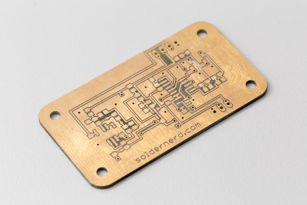
I recently ordered my first PCB at dirtypcbs.com and the result was promising. So there was nothing stopping me from finalizing the Rev B of my standalone Ultrasonic Anemometer and ordering a protopack. I’ve placed the order a few days ago and expect the boards to arrive here in 2 to 3 weeks. This should be good news for all those of you who have been asking for kits and want to contribute to the further developement of this project. I’ll build up one or two boards as soon as they get here and do some testing. If everything works as planned I can order some more components and ship some kits soon after that.

So today I’ll go through the changes I’ve made compared to the previous version. All in all the changes are quite minor and only require minimal changes in software. But let’s go through them one by one.

Non-volatile memory

This is the biggest change from a functional point of view. The PIC32MX250 doesn’t have any EEPROM memory of its own. So in order to be able to save some settings an the like I’ve added a Microchip 24AA16 I2C EEPROM providing 16kbit (2kB) of non-volatile memory. That should be more than enough to store any settings and calibrations one might want to make. For example, this gives the user the possibility to calibrate the filter kernels to the transducers used. Of course, the software first needs to make use of that memory but I think it’s great to have the possibility to durably store a reasonably large amount of data.

Support for 5V I2C communication

I’ve hinted at this in a previous post. On the Rev A board the I2C signals were pulled up to the 3.3 volt rail. This was great as long as one didn’t want to interface to a 5V device such as an Arduino. The microcontroller pins are 5V compatible so you want to be able to pull those lines up to 5V whenever you interface to a 5V device. So I’ve added a diode to allow the SDA and SCL lines to be pulled higher than 3.3 volts. The I2C reference voltage of 3.3 volts minus a schottky diode drop or about 3.1 volts is accessible from the I2C header at the bottom. So just connect that to the external device’s 5V operating voltage and you have a fully compliant 5V I2C bus.

Physical layout and connectors

There was a rather large 8-pin connector on the last version to connect to the transducers. Now all the connectors along the edges of the board are standard 100-mil headers. This also allowed me to slightly shrink the physical size of the board to 60x70mm.

The pinout has also slightly changed. The board is now powered from a header on the right-upper side and all three voltage rails are now externally accessible from a newly added header on the right side. The pin order on the I2C and SPI headers on the bottom side of the board has changed, mainly to accomodate an exteral I2C reference voltage.

Power supply

The tiny (SOT23-5) 3.3 volt linear regulator on the last version worked well but got rather hot when providing close to 50mA from a 12V input voltage. I never had any issues with it at room temperature but decided to be cautious and upgrade to a LD1117 regulator in a much larger SOT223 package. This should be more than sufficient any reasonable ambient temperature..

Miscellaneous changes

I changed the digipot used to set the amplifier gain to a Microchip MCP4531. This model only has 128 steps but this is still more than sufficient for its task and it’s quite a bit cheaper than the 256-step version.

I also had to change the crystal because the model previously used became unavailable.

That’s it for now. I’ll let you know as soon as the boards get here.

Arduino Ultrasonic Anemometer, DIY projects, General

Ultrasonic Anemometer Part 24: New Microcontroller and Software Controlled Gain

2016-06-27 Lukas Fässler 1 Comment

It’s been almost three weeks since my last post and some further progress has been made. I’ve upgraded the microcontroller and can now control the gain of the second amplifier stage in software. But let’s look at the changes in some more detail.

New microcontroller: PIC32MX250

I mentioned last time that I was running out of code space, i.e. flash memory on the PIC32MC220. That particular model has only 32k of flash and I’m using the free version of the XC32 compiler. That free version only performs limited amounts of optimization and therefore produces rather large and slow code compared to the standard and professional version. But the other two are rather costly (around USD 500 and 1000, respectively) and are not really an option here. And at least so far I’ve always had all the speed I needed so the only issue was flash memory.

So the straight forward solution was to upgrade the microcontroller to an otherwise identical model with more memory. The 250 I’m using now has four times more of both flash (now 128k) and ram (now 32k). I unsoldered the old chip using a hot air gun and soldered in a PIC32MX250 in its place. Now we have all the flash we need to continue our journey.

Getting I2C to work

My design uses a dual op amp for the necessary amplification of the received signal. The first stage is ground-referenced and uses a simple resistive divider to set the gain (currently set at 11).

The second stage is biased to 1.65V (i.e. half way between ground and 3.3 volts) and has its gain controlled by a I2C digipot. The idea is to have the PIC control the digipot so it can adjust the gain as needed to compensate for any effect that might change the amplitude of the received signal.

So in order to control our digipot we first need to get the I2C interface working on the PIC. There are two (identical) I2C peripherals on the PIC32MX2xx and this design uses one of them (#2) exclusively to communicate to the digipot. The other one (#1) is then available to interface to the outside world.

I’ve written a set of simple functions to use the I2C interface. So far I’ve only implemented master transmit mode since that’s the only thing we need here.

void app_i2c_internal_init(void);
bool app_i2c_internal_write(uint8_t address, uint8_t *data, uint8_t length);
void app_i2c_internal_writeDigipot(uint8_t value);

The functions are entirely non-blocking so they can be called from within the interrupt service routines that do the measurement.

Fixing a design bug

Unfortunately, I made a mistake in the schematic when I referenced the feedback loop of the second op amp stage to ground instead of the mentioned 1.65 volts. Now let’s look at what that did to the signal. First, below is the signal with the digipot at 0 (of 256). The gain is set to one and all is well.

But at a setting of 64, some clipping starts to occur as shown below.

With the gain turned up to 4 with a digipot setting of 192 things get really uggly with a completely unrecognizable output signal.

I was extremely lucky that the correct signal was available right next to the pin where I needed it so all I had to do was to cut the ground connection with a carving knife and to connect the correct signal using a tiny bit of wire. The change is hardly visible on the photo below. Can you spot it? It’s almost at the center of the photo at pin 5 (bottom right) of the small 8-pin IC. It now connects to the 10k resistor at the bottom instead of the ground plane on its right.

Controlling the gain in software

With that error fixed we can now set the gain as we please. Here some examples. Yellow is the (unamplified) input signal whereas green is the output of the (fixed) first amplifier stage. The purple signal is calculated as the difference between the DAC+ and DAC- signals. Those two signals is what we feed into the PIC to be measured.

With the gain at 1 (digipot at 0) we get a about 2.6 volts peak-peak. A bit little but sufficient.

This is probably about what we want. Digipot at 50 resulting in a peak-peak amplitude of a bit above 3 volts.

Needless to say that we can jerk the gain up far more than that if we want. Below is an example where a gain of 4 results in a seriously clipped signal.

Now let’s look a a situation where such a high gain might actually be useful. In the example below I’ve lowered the input voltage to only 5 volts. As a result the received signal is only 90mV in amplitude instead of the 220mV seen above. That’s easily compensated with a bit of help from our digipot. With a setting of 170 we get a nice, clean 3 volt output signal.

Calculating the necessary gain

For the examples above I’ve explicitly set the gain in the code. But what we really want is to have the software calculate and set the necessary gain automatically.

So I’ve implemented a simple algorithm to do so. I set some target value for the peak-to-peak amplitude of the signal measured by the DAC. Knowing the amplitude and digipot setting of the last measurement I calculate the optimal gain and digipot setting for the next measurement.

Above is the signal without this automatic gain setting in place (gain=1). As you can see, the peak-to-peak amplitudes vary quite a bit between transducer pairs. So the gain calculations, too, work on a transducer pair basis. Each direction gets its own setting to compensate for different transducer sensitivities.

Below is a screenshot of the result. Notice how now all transducer pairs have identical (and somewhat larger) amplitudes.

That’s it for today. Click here for my next post.

Arduino Ultrasonic Anemometer, DIY projects

Ultrasonic Anemometer Part 23: First successful measurements

2016-06-07 Lukas Fässler 16 Comments

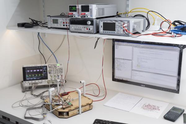
In my last post I was happy to report that I managed to get the USB interface to work. This interface has since proved to be extremely valuable in software development and testing. While the device is taking measurements you can look at the results (or intermediate results) at your PC in real time. You can even log large amounts of data to a .csv file and inspect the results in Excel.

But let’s look at the developements in a bit more detail. Last time the device was sending pulses and capturing some of the resulting zero-crossings but not much more than that. And in a not very structured way.

Measuring amplitude

Now it’s not only capturing the times when the zero-crossings occur but also measures the amplitude of the half-waves in between. In order to do that an interrupt is generated at every zero-crossing capture. Inside that interrupt service routine time of the zero-crossing is saved (as previously) and the ADC is started. In order to measure the amplitude at its maximum (or minimum in case of a negative half-wave), the ADC first samples the input for a 6.25 microseconds (which corresponds to a quarter-wave at 40kHz). I’ve chosen the sampling period slightly shorter to compensate for the time from when the zero-crossing occured unil the ADC is started. After the sampling period the internal sample-and-hold amplifier switches from sample to hold and the actual analog-to-digital conversion takes place.

The PIC’s datasheet advertises a maximum sampling rate of 1 million samples per second. Beware, though, that this requires separate Vref+ and Vref- connections and doesn’t work in differential mode anyway. In my configuration without separate analog references and differential measurements the maximum sampling rate drops to 400k samples per second. And the reported conversion time doesn’t include the sampling time yet. I wasn’t aware of that but luckily the PIC’s ADC is still more than fast enough for what I’m doing here.

Finding the absolute phase

Capturing the zero-crossings is relatively easy and the results are very precise. But there’s a challenge: there are hundreds of zero crossings for each burst of pulses sent. How do you know which zero-crossings to use?

The Arduino-based anemometer used an analog envelope detector to solve this problem. After averaging plenty of samples this works most of the time. But even after many attempts to tweek the analog circuit the envelope detector approach was never as reliable as I wanted it to be.

My standalone anemometer has an entirely different approach. Being able to digitally measure the amplitude of each half-wave we can tackle the challenge in software. We have a series of measurements and we have an idea of that the signal we are looking for looks like. Looking the scope screenshot below you could easily and reliably determine where the maximum amplitude occurs. That’s what we need to teach the software to do.

One could, of course, just loop through the all the amplitudes and find the maximum. But there are a lot of similar amplitudes and so any noise would make the result unreliable.

I did a bit of reading on digital signal processing (DSP) and realized that this is a classic DSP problem. The solution is a matched filter. You take the signal you are looking for (also known as kernel or template) and multiply it sample by sample with the captured signal and sum up the results. Do that for every possible (or reasonable) overlap of signal and kernel and find the position where the result reaches its maximum.

If you’re new to the subject (like I am), Steven W. Smith’s Digital Signal Processing is a great place to start. It’s even available online for free at dspguide.com. The method is also referred as convolution or correlation depending on who you ask. This wikipedia article gives a nice introduction to the subject.

Implementing the matched filter

I’ve parameterized the software to capture 34 zero crossings as well as the n=33 amplitudes in between them. The kernel consists of k=17 data points with a peak in the middle.

There are n-k+1=17 possibilities to entirely overlap the kernel with the signal. We can skip all the odd numbers where a negative kernel value would be multiplied with a positive sample value and vice versa. This leaves us with 9 possible positions to chose from.

For each position we need to do 17 multiplications and 16 additions. And we need to do that for every single measurement, i.e. 512 times per second. That sounds like a lot of work and it probably is. Luckily, since this is a very common DSP task, microcontrollers like the PIC32 have a special instruction for this. It’s called MAC – Multiply Accumulate and executes in a single clock cycle. The result is just amazing. The corresponding ISR takes less than 30 microseconds, including some housekeeping tasks as can be seen in the screenshot below.

Once the maximum amplitude is found, the 16 zero-crossings around it (i.e. the 8 before and the 8 after) are summed up and the sum is saved as the result of that measurement.

Averaging measurements

The goal is to report wind speed and temperature four times per second. Since there are 512 measurements per second we can use up to 128 individual measurements (32 in each direction) to do our calculations.

So we have plenty of data to identify and exclude outliers and do some averaging of the remaining samples. Robust statistics is the key word here, click here for the corresponding wikipedia article.

For now I’m doing something reasonably simple: First the 32 results per direction are sorted. The 12 lowest and 12 highest results are ignored and only the 8 results in the middle are summed up.

This might seem wasteful but it makes the average very robust against outliers and still results in 16 x 8 = 128 zero-crossings being averaged. The resolution of each zero-crossing is equal to 1 / 48MHz or about 20.83 nanoseconds. Summing up 128 of them gives us a resolution of far below a nanosecond. Beware however that resolution doesn not imply accuracy.

As a last step, the resulting sum is multiplied with 125 and then divided by 768 to make the unit 1 nanosecond. So every 250 milliseconds we finally have 4 time-of-flight measurements with a resolution of 1 nanosecond. That’s what we will use to calculate the winds speed as well as wind direction and temperature.

This sorting and averaging step is a bit more costly in terms of computation time. It takes around 600 microseconds to complete (see below). But unlike the convolution, it only has to be performed 4 times per second so this is more than fine.

Calculating wind speed

We are finally in a position to calculate the actual wind speed. There are various ways of doing this. For now I’ve just done the simple approach of taking the difference in time-of-flight, assuming room temperature and solving for wind speed. This means solving a quadratic equation for which I have resorted to floating point math and using <math.h> for the square root function.

I don’t have my wind tunnel any more so doing any testing was difficult. But one thing was soon obvious: at zero wind speed, the time-of-flight measurements match extremely well and are extrordinary stable from measurement to measurement. Also, looking at the intermediate results (i.e. the 128 single measurements before averaging) shows that there are basically no outliers present. I could randomly pick a measurement and still get a very reasonable value.

Something seems to be systematically wrong with the first of the 128 measurements but I haven’t had time to look into this. Otherwise, the results are impressively stable. And I’m only using a relatively primitive kernel for the matched filter.

USB data logging

As I’ve mentioned at the beginning, the USB interface lets me do some serious data logging even at this early stage of development. Here’s a list of what I can do by sending a character to the device from a USB terminal.

‘Z’: Get all the 34 zero-crossings of a single measurement
‘A’: Get all 33 amplitudes of a single measurement
‘F’: Get a full single measurement, i.e. 34 zero-crossings plus 33 amplitudes
‘T’: Get all the 4 x 32 = 128 time-of-flights for a measurement series
‘R’: Get the 4 averaged time-of-flights as well as wind speed and temperature

Some versions of these commands also let you specify the direction you’re interested in as well as how many sets of data you want to receive. This makes it easy to log large amounts of data that you can use to test possible algorithms on your PC before you implement them on the PIC.

Next steps

The next step is to get the I2C digipot working so I can control the amplification in software. My idea is to aim for a maximum amplitude of around 3 volts independent of wind speed and so on.

There’s also plenty of work to do to improve the algorithm that calculates wind speed and temperature. And then I also have to implement the I2C and SPI interfaces that let the anemometer communicate to other embedded devices like an Arduino or Raspberry Pi.

Having used floating point math and <math.h> I’m also running out of flash memory. I’m currently using 93% of flash (32kB total) and 52% of ram (8kB total). There will be a slightly revised board (Rev B) that uses a PIC32MX250 which is identical to the MX220 used here but has four times as much flash and ram.

That’s it for today. On the overview page you find the software at the stage of developement just described as well as some examples of logged data (all at zero wind speed) as .csv files.

The next post on this project is here: Part 24.

Arduino Ultrasonic Anemometer, DIY projects, Uncategorized

Ultrasonic Anemometer Part 22: USB up and running

2016-05-29 Lukas Fässler 3 Comments

Last time I showed you the nice new hardware of the new standalone ultrasonic anemometer. But at that time I had hardly any software written for it so I couldn’t do much with its 32 bit microcontroller. So the last two or three weeks I spend lots of time writing code that I’d like to share with you today.

As I mentioned last time I worried most about getting the USB working properly. All the bit-fiddling with timers, PWM modules, input capture modules and the like can be time consuming and at time even frustrating. But I have all the confidence that I finally get what I aimed for. It might take a few nights digging through data sheets but in the end it will almost definitely work.

Now with USB I don’t quite have that level of confidence. The USB specification is quite overwhelming and there are almost countless registers to properly set and USB descriptors to specify. Without some sample code I’m pretty much lost I must admit.

Outdated Application Notes

So I was happy to see that Microchip has published a number of application notes and accompanying software. A handful of .h and .c files that you can include in your project, change some settings to suit your particular application and you’re ready to go. At least that’s what I thought.

All those application notes were published around 2008 and the code they are referring to is nowhere to be found nowadays. Aparently, Microchip has been quite pushy trying to get their PIC32 customers migrate to their new library or rather framework called Harmony. MPLAB no longer even includes the the PLIB peripheral library everyone has been using for decades. Microchip has depreciated it and while you can still download it they make very clear that Harmony is the library of the future.

On the road with MPLAB Harmony

So faced with few other alternatives I turned to the aforementioned Harmony library. It’s many hundred megabytes to download and takes up almost two gigabytes of disk space. It integrates nicely into MPLAB X and so I created a first project. You can graphically configure the clock and pin settings so I did that. Clicked on ‘create code’ and was nothing less than shocked by the code I got. Around a dozend source files scattered around in a dozend deeply nested folders and subfolders. And that was not yet it. Those files referenced dozends more files that came as part of harmony. It took me quite a while to just more or less figure out what the project was doing. And it didn’t do anything yet except setting some clock and port settings. Just a nightmare.

But I felt I had few other options so I continued with harmony anyway. And after a few hours I had an almost working USB device. It enumerated just fine but I couldn’t send any data from or to it. It took me more than a week to finally get it working. In the end it was just a single character: a 1 instead of a 2 in one of the configuration files. But until then I had spent a lot of time with that harmony code and was forced to read through a lot of its documentation which is worth thousands uppon thousands of pages of PDFs.

So USB was finally working and I had acquired some rudimentary understanding of MPLAB Harmony. I still hated the whole framework but I thought that I now understand it well enough to change the code to suit my taste. So I spent another few nights trying to do that until it dawned on me that this is leading nowhere. Fortunately, by that time I had read and learned some more about Harmony and was willing to give it another try working with it as opposed to against it. So for the last week or so I was doing that.

And while I still don’t love everyting about it I now feel comfortable working with that library. I’ve tried to follow its conventions and recommendations even where they didn’t make too much sense to me. I think this will make it much easier for others to work with my code and chances are that the conventions and recommendations will start to make more sense as I get more familiar with the framework. And its nice to know that I can integrate another module or migrate to another microcontroller without having to re-invent everything.

That was a long introduction but after all that pain the last few weeks I just had to write that down. Now to business.

USB

The anemometer inplements the USB HID (human interface device) class. While mainly aimed at devices such as mice and keyboards, this USB device sees a lot of use in applications that have nothing to do with human interaction. You can transfer up to 64 kbytes of data (64 bytes every millisecond) in each direction with guaranteed latency and that’s plenty for many applications. That data can be anything and in any format you like. And the good thing is that you don’t need to write your own drivers. You can free-ride on the device drivers that came with the operating system just like you don’t need to install a driver when you attach a new keyboard to your computer.

I’ve written a bit of code on top of the Harmony library to provide the main application with a simple to use interface. It nicely encapsulates the the USB logic and data and adds a bit of buffering functionality on top of that. It’s just two files: app_usb.h and app_usb.c in the app_usb subfolder. You can basically include them in your project and they handle all the USB stuff for you.

Once initialized, the necessary code runns inside an interrupt service routine (ISR) so the main application has nothing to worry about. All the USB data including the data buffers are private to the app_usb.c file. The app_usb.h defines just 8 simple, non-blocking functions:

void app_usb_init(void);
bool app_usb_isReady(void);
uint8_t* app_usb_getReceiveBuffer(void);
uint8_t app_usb_getReceiveBufferCount(void);
uint8_t* app_usb_getTransmitBuffer(void);
uint8_t app_usb_getTransmitBufferCount(void);
void app_usb_freeReceiveBuffer(void);
void app_usb_sendTransmitBuffer(void);

At system initialization you call app_usb_init(). But you can’t expect to have an USB connection. You need to check app_usb_isReady() every time. You never know if there is a USB cable plugged in and even if you had a connection that cable might be unplugged at any time. The module handles all that hot plugging/unplugging gracefully.

The module implements a circular buffer for both received packages (aka frames) and packages to be sent. Each package is 64 bytes in size and the ring buffers can be set at compile time but must be a power of 2. Currently the receive buffer consists of 4 frames and the transmit buffer of 8 frames.

The app_usb_getReceiveBufferCount() informs the caller how many new USB frames have been received if any. app_usb_getReceiveBuffer() then returns a handle to the first received frame. FIFO – First In First Out. Once the frame is no longer needed the application calls app_usb_freeReceiveBuffer() and the buffer can be re-used.

Sending data works similarly simple. app_usb_getTransmitBufferCount() returns the number of transmit buffers currently in use. If this number is smaller than then number of buffers then more data transmissions can be scheduled. Get a handle to then next buffer by calling app_usb_getTransmitBuffer(), write the data to be sent to the buffer and then call app_usb_sendTransmitBuffer().

Taking measurements

This way the main application can focus on more interesting tasks such as measuring wind speed and direction. The first task for doing so is sending some pulses.

If you’ve alredy followed this project for a while you are probably familiar with the kind of screenshot above. Bursts of a PWM signal at 40kHz (SIGNAL, red) are sent trough ultrasonic transducers. Note that the signal is now active-low (i.e. inverted) since the mosfet drivers used to drive the transducers are themselfs inverting.

As before, the DIRECTION and AXIS signal determine which transducer is transmitting and receving. The SCLK and MOSI signals are just used for debugging purposes for now. They indicate when an ISR is running which helps a lot since in this example ALL the code is running inside an ISR.

TimeZero

As you can see above, the AXIS and DIRECTION signals are set a few microseconds before we start sending pulses. The first edge of the burst occurs when the 32 bit-timer (consisting of the 16-bit timers TMR2 and TMR3) is cleared. This is the point in time all our measurements are referenced to. The timer runs at the full CPU clock of 48Mhz so the resolution is about 20.8 nanoseconds.

Output Compare module 2 (OC2) handles the PWM pulses. Currently each burst consists of 12 pulses. At 48MHz a full wave equals 1200 clock cycles as opposed to 400 on the Arduino previously used. Note that the frequency of the pulses is precisely 40kHz as expected and that very little time is spend in ISRs despite the unoptimized C code.

The timer overflows precisely 512 times per second so each measurement takes a little less than 2 milliseconds. Output compare module 1 (OC1) can be used to generate an interrupt at any time during that interval. Currently it does three things: It takes care of the AXIS and DIRECTION signals which are set just shortly before the timer overflows. It also triggers the measurements of the zero-crossings and cancels them if they don’t complete withing reasonable time.

The input capture module 4 (IC4) captures the zero-crossings of the received and amplified signal. The board contains a high speed comparator to detect these events so the microcontroller only needs to measure the precise time whn they occur. The IC4 module has an internal buffer so we don’t need to generate an interrupt after every capture. I’ve currently set things up so that an interrupt occurs after 4 values have been captured up to a total of 32 measurements.

Commicating the results over USB

In order to find the wind speed and direction we need to somehow identify the peak in the received signal which is where the ADC comes in. But I think this is enough for now and I instead show you how the measurements taken so far can be sent to a PC via USB.

The board doesn’t have any display or anything to communicate with a human. There’s not even a status LED we could blink. That would have been nice but there are just not enough I/O pins unfortunately. So connecting the board to a PC via USB is a straight-forward way of communicating with this device. Actually, USB will be the main testing and debugging tool during development. The in-circuit debugger isn’t very useful in this application since the measurements have to happen in real time. Setting breakpoints will just mess things up.That’s why I insisted to get USB working first.

I’ve downloaded a simple terminal called YAT (yet another termial) that allows me to easily talk to the anemometer board. The anemometer looks at the first character in any message sent from the host and then decides what to do. So far I’ve implemented:

‘T’: Return the current value of the 32-bit timer
‘Z’: Return axis (0/1), direction(0/1), measurement count (0-31) values as well as the results of the first 9 zero-crossing measurements
Anything else: Echo back the received string

Here’s what my chat with the Standalone Ultrasonic Anemomete looked like.

Of course, the measurement is far from complete at this stage but I think this is a nice foundation to build uppon. The code is quite clean for this early stage of development and being able to communicate with the device in real-time over USB is really a great advantage.

The software can be downloaded on the project over view page and as always I appreciate any feedback.

The next post on this project can be found here.

Arduino Ultrasonic Anemometer, DIY projects

Ultrasonic Anemometer Part 21: Standalone Anemometer Hardware

2016-05-14 Lukas Fässler 1 Comment

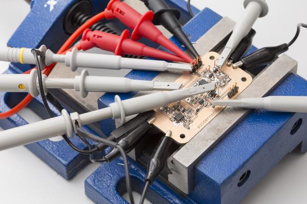
Last time I went through the design of my new standalone anemometer. Now it’s time to build this thing and see if it works as planned.

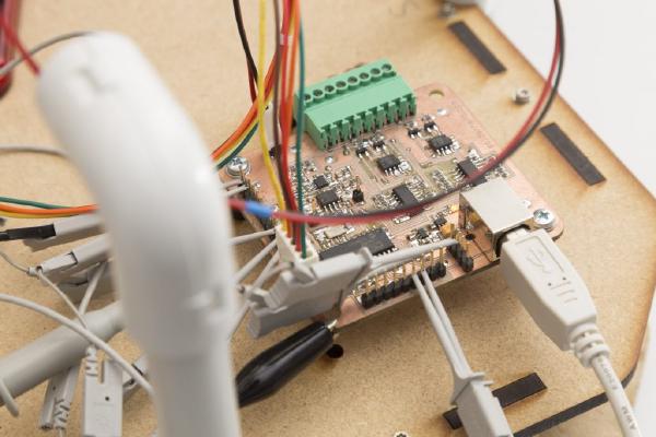
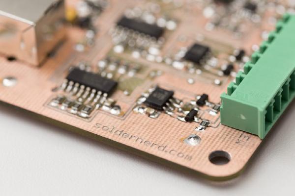
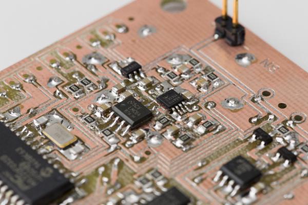
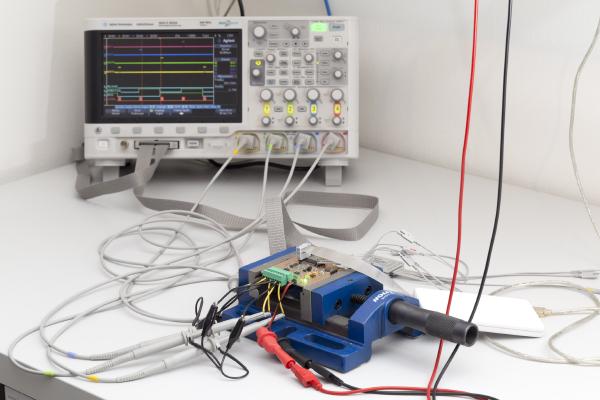
After I fried a couple of chips on my driver circuit testing board due to a wrong chip in the power supply I was a bit more careful this time and built up the board step by step.

Only after I confirmed that the power supply was ok I dared to solder some more.

The next step was to add the PIC32 with the crystal, the programming header and all the caps they need. This is a chip family that I’ve never used before so I wanted to first see if I can program it. All went well and I managed to get it to run on the crystal’s 8MHz boosted up to 40MHz by an internal PLL. So I was ready for the rest.

I wrote some very basic software and confirmed that at least the basics were working ok. I was able to send and receive pulses, the pulses got amplified, the zero-crossing detector worked and so forth.

As mentioned, I’m entirely new to the PIC32 microcontroller series. There are a lot of similarities to the PIC16 and PIC18 series that I’m quite familiar with but still it’s always a challenge to work with a new family of chips and the tools that come with it. I took me the better part of an afternoon to master the vectored interrupts with the different priority levels and so on.

20160428_StandaloneAnemometer_040 — Driver circuit (front) and standalone anemometer (back) side by side.

By the way, with this project I’m using the free MPLAB X IDE with the also free XC32 C compiler from Microchip. So anyone is able to write, modify or compile code for this thing with free software. At least at the moment you need a programmer to actually burn the chip. But the PICkit3 only costs around 50 dollars and my idea is to write a USB bootloader so that any user can modify the software of a pre-programmed board.

So now comes what I think might be the hardest part: Getting the USB to work. I’ve spent quite a few hours so far but haven’t managed to get it working properly yet. If anyone has experience with this kind of software development – Let me know, any help is highly appreciated.

It now works: Click here to view it.

Arduino Ultrasonic Anemometer, DIY projects

Ultrasonic Anemometer Part 20: Standalone Anemometer Design

2016-05-11 Lukas Fässler 2 Comments

Last time I outlined my reasons to ‘go digital’ by adding a powerful on-board microcontroller and designing a standalone wind meter.

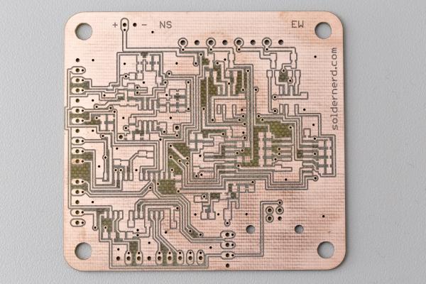
In the weeks that followed that decision I tried to find a suitable microcontroller and to design a prototype. Today I’ll show you the result of that work.

I looked at various series of microcontrollers from different manufacturers and finally decided to go for the Microchip PIC32 series. It offers everything I could possibly ask for: 32 bit architecture, inexpensive, vectored interrupts, integer division, any interface you want (depending on the model of course) , available in large, low pin count, hobbyist friendly packages and so on.

As you can see above, the model chosen for my prototype is a PIC32MX220. This is low to mid-end representative of this series but even so the specs are quite impressive. CPU clock up to 50MHz, one instruction per clock cycle, full-speed USB 2.0, 32kB flash, 8kB RAM and all of that in a SOIC28 package at a price of CHF 3.58 in single quantities.

After having chosen a chip the next task was to come up with an actual design. I took my anemometer driver design and tried to integrated the new PIC32. That driver circuit had performed extraordinary well so I changed very little. I left away the RELEASE signal since my tests had shown it to be unnecessary. I also replaced the LM5111-1M mosfet drivers by LM5111-2M. The difference is that the 2M is inverting while the 1M is not. The reason for changing this is because the 2M is available at a significantly lower price of CHF 1.35 vs CHF 2.25. Not a big deal if you just build a single prototype but I thought it might be smart to change this anyway. This also required some resistors to be changed from pull-downs to pull-ups. Except these details everything stayed the same with the drive circuit.

I also had to re-design the power supply since the PIC needs a 3.3 volt rail as opposed to 5 volts in the driver test circuit. Since I had to re-design it anyway I also downsized the power supply somewhat. I’ve otherwise resisted all temptations to use smaller components but the power supply was just a bit too big with the two SOIC8 chips and four size C tantalum caps.

The prototype now uses an MCP1755 linear 3.3V regulator in a SOT23-5 package with a 33uF size B tantalum cap at its input and a 10uF 0805 size ceramic cap at the output. A TCM829 (also in a SOT23-5 package) and two more 10uF caps produce the -3.3 volts output. So there is a total of three supply rails: +12V, +3.3V and -3.3V.

A major challenge was to make do with the very limited number of I/O pins on the PIC. 28 pins seem like a lot for the task at hand but plenty of them are already used for things like supply voltages and the like.

In the end I managed to still get three independent interfaces to the outside world: USB 2.0, I2C and SPI. All these interfaces as well as just about any other signal of interest is easily accessible from one of the numerous 100mil headers along the edges of the board.

The amplifier still uses a LMC6482 dual op amp , now running on a+/- 3.3 volt supply. The first stage amplifies the ground-referenced input signal by a fixed factor (currently 11 but this might change). The output signal is then biased to 1.65 volts and amplified once again. This time the gain can be adjusted digitally via a MCP4561 I2C digipot.

Before I forget: The PIC gets its system clock from a 8MHz crystal. That might seem low but there are two (variable) PLLs inside the PIC that (together with a number of pre- and post-scalers) let us produce the 48Mhz signal needed for USB as well as a reasonable clock speed to run the CPU and peripheral bus on (probably also 48MHz but we’ll see).

The board layout proved to be a bit tricky because there isn’t that much space on the board and I had quite clear ideas where I wanted certain headers to be. So I was more than happy when all the traces were finally laid out.

As you can see, the PCB is already milled and the vias soldered. I can’t wait to build this thing up and start to do some programming. That will be the topic of my next post.

As always, a zip file with the eagle files and PDFs of the schematic and board layout can be found on the overivew page.

And here‘s the finished board.

Arduino Ultrasonic Anemometer, DIY projects

Ultrasonic Anemometer Part 19: Testing the Analog Circuit

2016-04-26 Lukas Fässler 5 Comments

In my last post I went through the design of the analog part of the ultrasonic anemometer. Today we will see how the circuit designed last time performs in practice.

Active Full Wave Rectifier

Let’s first look at the active full-wave rectifier. As a first test I fed the input with a 40kHz sine wave from the scope’s signal generator. Here’s what I got to see on the scope.

The input signal is shown in yellow. The pink signal is calculated as the absolute value of the input and is what we are trying to archieve. Finally, the blue signal shows what we actually get on the rectifier’s output. What do you think? The basic wave form is obviously right but the precision leaves quite something to be desired. So I tried the same setup with an input signal 10 times slower, i.e. 4kHz.

As you can easily see, things look much better at 4kHz. That doesn’t make it much better for us since we need it to operate at 40kHz but there doesn’t seem to be anything fundamentally wrong with the design per-se. I think a faster op amp might be that is needed to make this thing work properly at 40kHz, too.

Zero-Crossing Detector

The zero-crossing detector is by far the simplest element of this circuit and has hardly changed since the Arduino anemometer shield. It’s output is shown in blue above. It works just as expected, no surprise here. Well, in the end it’s just a comparator so the sources for error are limited.

Peak Detector Sample And Hold

The input to the peak detector is the rectifier’s output so we should expect to see at least some inaccuracy carried over from the rectifier.

Below is what I got. Again, yellow is the 40kHz sine wave input. Blue and red are the peak detector of the positive and negative half-wave, respectively. Green is the output, i.e. either the blue or red singnal as chosen by the 2:1 multiplexer.

The good news is that the circuit basically works as designed. Each peak detector gets zeroed at just the right time. From the screen shot above one might even conclude that the peak detector is fairly accurate. Both half-waves show very similar amplitudes and the output is nicely held stable during the hold period. No droop is visible at least at this level of magnification.

Once you zoom in, things start to look less pretty. There is in deed no droop but the opposite. The output signal rises during the hold period. If you look closely in the screen shot above you can even see it – the segments of the green signal are slightly rising. We’re talking maybe 10mV here, far from dramatic but still.

Conclusion

My conclusion is as follows:

Zero crossing detector: perfect
Active rectifier: poor performance as is but can probably be fixed with a faster op-amp.
Peak detector: ok but not good enough. might need lots of trial-and-error to improve it.

I have mentioned in a previous post that I’m still unsure if I should stick to the predominantly analog signal processing or if I should make the switch to a more contemporary, digital, DSP like approach. After having spent an evening or two testing and tweeking this circuit the answer became clear – go digital.

If you’ve followed my blog for even just a short while you have likely noticed that I enjoy designing and building hardware. Probably more than I enjoy writing software. But there are several good reasons to to more in software and less in hardware when it comes to this project.

The circuit as described above works kind of. But it might take a loooong time to improve it until it really performs well. Chances are that it will never perform as well as I’d like it to.
Board space. All this circuitry takes up considerable board space. A later version might use smaller components but this thing will always take up quite a bit of space – maybe a third of the total board area.
Even with most of the heavy lifting done in hardware the Arduino is likely not fast enough. We’d need to sample the amplitude at 80kHz which is out of reach for the Arduino’s Atmega328 even when sacrificing some resolution.
Further development. Chosing a digital approach enables users to actively contribute to the further development and improvement of this project.
Versatility: Eqiping the anemometer with a dedicated microcontroller makes this project much more versatile. It no longer has to be Arduino specific. If you’re an Arduino lover I promise you it will always be Arduino compatible. No need to worry. But equiping it with a easy-to-use SPI or I2C interface makes it useful beyond the Arduino community.
Cost. My analog design uses two op amps among other things. Precision op amps are relatively costly components. It’s not an expensive circuit but it will always cost several dollars for the components alone. And improving the circuit is unlikely to make it cheaper.
Processing power is cheap. You might rightly say that a few bucks is not a lot of money to spend on some nice analog circuitry. I fully agree. But one can buy a lot of processing power for far less money nowadays.

Let me elaborate on some of these points:

Versatility: Arduino Only vs. Anyting, including Arduino

The arduino is a great platform with a great user community. But the Arduino Uno might not be the best choice for this project. A on board microcontroller gives user the option to use this anemometer from whatever platform they chose. Besides: An arduino is a very expensive device even when compared to a quite high-end microcontroller. 32-bit microcontrollers running at frequencies of 40MHz and higher are available for less than 2 or 3 dollars even in small (say, 10 pieces) quantities. More advanced models might cost, say, 5 dollars. In comparison, an Atmel Atmega328 as used on the Arduino currently costs CHF 3.10 (USD 3.18 at the time of writing) at Farnell. Not really value for money if you ask me.

Community Driven Developement

There are lots of creat coders out there. I can write decent code but there are plenty of people way better at that than I ever will be. I see this as an opportuinity to greatly improve this project. Once I get this thing up-and-running I’d like to build a small series and let users share their experience and contribute to the code. Have an idea on how it could be improved? Try it yourself if you have the skills. Share your code if it works. Or share your thoughts and ideas if writing emedded softwar is not for you. So the anemometer could get better and better without having to get new hardware. Just update the firmware.

Next steps

In the weeks to come I will work hard to find a suitable microcontroller and to design and build a board with all that is needed for a stand-alone ultrasonic anemometer.

It’s now ready, click here.

Arduino Ultrasonic Anemometer, DIY projects

Ultrasonic Anemometer Part 18: Analog Signal Processing

2016-04-19 Lukas Fässler 2 Comments

Recently, I’ve sucessfully tested the new driver ciruit for my ultrasonic anemometer. It performed even better than I expected and I will be happy to use it pretty much as it is.

By the way: If you want to get an overview over how this project has developed over time check out the overview page. If you’re more interested in my latest design, this link will take to my new attempt.

So we have a circuit that can send powerful ultrasonic pulses from the right transducer, receive the signal from the opposite transducer and route it through an amplifier. The next task is to tell the time-of-flight from the received signal. A contemporary approach would probably involve some sort of DSP and software. My last approach used some analog circuitery to detect the zero crossings as well as the envelope of the received signal. Since most of the heavy lifting was done in hardware, a simple 8-bit microcontroller like the one on the Arduino UNO could be used to do the measurements.

For my new approach I haven’t quite decided which route to take. To me they both have a certain appeal. And over the last year or so I’ve had quite some ideas on how to process the signal in hardware so I’ll give it a try and see how it works out. In this post I’ll go through this new circuit and explain how it works (or is supposed to work) step-by-step.

The zero crossing detector (ZCD) is almost identical to to my last design. The amplifier output is biased to half the positive supply voltage and fed into a fast comparator (Microchip MCP6561R). On the comparator’s output we get a precise digital signal indicating if we are currently looking at the positive or negative half-wave. Right at the logic edge we observe a zero crossing which can then be used to very precisely determine the phase shift relative to the transmitted singal.

The more challenging part is to tell the absolute phase – this is where my last project was only partly successful. It used an active low-pass filter to get the envelope of the received singal. This envelope was then compared to some threshold and the time from the transmition of the singal to when the envelope exceeded the threshold was measured. With plenty of averaging this gave a usable but far from perfect indication of absolute phase. So this time I’ll try something entirely new.

The amplified singal is first run trough an active full-wave rectifier as found on page 257 of Horowitz and Hill’s 3rd edition of Art of Electronics. It uses two op amps as well as some resistors and diodes to produce a singal that corresponds to the absolute value of its input. The two op amps come in a single package. It’s the same type as for the amplification stage of the driver circuit – a Texas LMC6482.

Now the rest of the circuit is a bit more adventurous. It attempts to produce a signal that corresponds to the peak of the previous half-wave. So it is steady during each halv-wave period and should give a (hopefully precise) indication of the amplitude of the received signal. This singal can then sampled by an ADC at 80kHz triggered by the zero crossing detector. 80kHz is not that fast for a (say) 10-bit ADC and definitely much slower than what we’d need if we sampled the amplified signal directly.

The advantage of measuring the amplitude is the following: We can find the peak of the amplitude in simple software and use the time when the peak occured to find the absolute phase. So we are no longer dependant on the absolute amplitude (as we were with the envelope detector approach) but only care about when the peak in amplitude occured. I think (hope) this is a much more reliable approach.

In order to find the peak of each half-wave I use a pair of simple diode-plus-capacitor peak detectors. One is held stable (“hold”) and fed through an op-amp buffer to minimize droop while the other is looking for the next peak (“sample”). At the beginning of the sample period the capacitor is discharged through a n-channel mosfet that is turned on for just an instance.

The whole mechanism is controlled by the output of the zero-crossing detector so absolutely no software intervention is needed to produce it. The microcontroller can just wait for the ZCD to trigger an interrupt (as before) and take a sample of the output.

The circuit is not that complex and used an inexpensive and readily available 74HC4053 multiplexer at its center. I don’t have any idea yet how this thing will perform but I must say this little circuit was a lot of fun to design.

Until my next post I will have built and tested this cuircuit and will let you know how it performs. Until then I leave you with the eagle files as well as PDFs of the schematic and layout as a zip file.

Here’s how the final circuit looks and how it performs: Part 19.

DIY projects

Temperature Controlled Fan

2016-04-09 Lukas Fässler 17 Comments

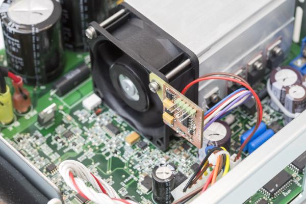
I’m currently mainly working on my new anemometer design but once in a while I get distracted. For example when my Keysight E3645A lab power supply was making so much noise that I could hardly concentrate. That’s when the idea of this fan controller was born.

Of course, the best temperature controlled fan in the world doesn’t help if you really need the cooling the fan is providing. But very often a small fraction of the cooling would do just fine most of the time. In my case the supply does control the speed of the fan. But it doesn’t seem to measure the temperature at all but seems to calculate the necessary cooling in a worst-case condition. An for a supply that may be rack-mounted together with lots of other heat dissipating gear the worst-case might be quite demanding. But my supply just sits on a shelf at, say, 22 degrees ambiant. And most of the time I’m hardly pulling any current. When working with microcontroller designs it’s rare for me to pull more than a few tens of milliamps. So little cooling is needed most of the time. But the E3645A (this one here does a better job) ran its fan at crazy speeds while the case still had this cold metallic feel to it. So we can definitely do better.

So the first step was to open the supply and to see what kind of fan it uses and how it is controlled. After beaking some seals and opening the case I found a 60x60x25mm 12V fan of Chinese origin. I also found out that the supply uses linear control. So there’s no PWM or anything but the supply voltage just varies in (I think) four steps from 7.4 to 12 volts. Most surprisingly, this voltage is not ground-referenced but symmetric around ground, i.e. plus/minus 6 volts.

I was pleased to see that the fan connects to the main board by means of a standard two-pin 100mil header. So I could just plug anything in between the board and the fan.

That’s exactly what my first idea was. Stick with the original fan and just put a PWM controller in between. I’ve just recently made some LED dimmers and the technology needed here seemed to be very similar. So Rev A of my fan controller was born.

It’s simple: A linear 5V regulator, a PIC16F18325 microcontroller, an LMT86 temperature sensor and a N-channel mosfet. The PIC chosen here runs at up to 32MHz on an internal oscillator, has an internal voltage reference (of 1.024, 2.048 or 4.096V), six PWM modules and plenty of other nice features while comming in a small 14-pin package. So all I need to do is to measure the temperature, calculate the desired fan speed and set the PWM duty cycle accordingly.

My first surprise came when I first wanted to program the PIC. My trusted Mikroelectronika MikroC for PIC compiler doesn’t know that chip. And neither does my MikroProg programmer. So after a little bit of research I ordered a PICkit3 and downloaded the MPLAB IDE. As a nice side effect I can now also compile code for and program the fancier PICs like the DSPics and PIC32s. I might do that before long.

So I did the necessary programming (and debugging) and attached a small fan. It all worked but I had to chose a quite low PWM frequency in order to make the fan spin at lower duty cycles. And probably as a result of the low PWM frequency the motion of the fan didn’t look or sound very smooth.

With the larger fan from the supply things only got worse. I had to lower the PWM frequency even more into the tens of Hz range so it would spin at all. And even like this I couldn’t get it to run at low duty cycles. Of course, the low frequency caused nasty vibrations so I gave up on this approach. I read online that other people successfully use PWM on their fans but at least this model wasn’t happy to be PWM-dimmed. Does anybody know more about this? Was this an option in the old days before brushless motors were the norm? Is it that brushless motors aren’t unsuitable for this kind of control alltogether or does it depend on the specific model? Please use the comments section below if you can shead some light on this.

But I don’t give up easily so after a bit of research I ordered a four-wire fan conforming to the so-called Intel spec. Besides ground and +12V they have two control lines. A PWM line that lets you control the fan speed by means of a (25kHz nominally) PWM singal. And a so-called TACH singal that allows you to read the current fan speed. The PWM line has internal pull-ups to (depending on the fan) 3.3 or 5 volts so you just need to pull it low. The TACH signal needs an external pull-up resistor and gets pulled low by the fan twice per revolution. So you’re getting a digital signal with a frequency of twice the fan speed.

I ordered a EBM Papst 622/2 HHP which is the right size and somewhat more powerful than the original fan. The new board has a somewhat odd shape so I can use one of the fan’s mounting screws to mount the board as well. Note that all the copper has been removed around the mounting hole. The fan is attached to a heat sink which is grounded while our board runs on a split suply. So ground as our board sees it is not actually ground but a negative voltage so we have to be careful.

The new Rev B design runs on 3.3 volts in order to be compatible with any fan independent of the fan’s internal logic voltage. I’ve also used a different temperature sensor – a classic LM35.

Like the Rev A there is an LED to visually indicate what’s going on. There are also three pins on the microcontroller that are intended to be used as debug pins so I put some vias there to make it easy to connect a scope probe.

Above you get an idea of what the TACH signal looks like. It’s a quite low frequency singal since there are only two pulses per rotation. So the measured 104Hz shown on the screenshot correspond to 3120 RPM.

Having a TACH signal to measure and three debug outputs to worry about made the software development somewhat more involved but it was well worth it. I’ve used the debug pins as follows:

Actual (i.e. mesured) fan speed. 100% corresponds to 10000RPM
Target fan speed. 100% corresponds to 10000RPM
Measured temperature. 100% corresponds to 100 degrees centigrade

So from the duty cycle measured by a scope you can easily read the speeds and temperature.

Of course this is only possible since there are some unused PWM modules left. But as I said, this PIC has 6 of them and only two are needed to measure the fan speed and another to control the fan.

The transfer function from temperature to fan speed can be freely defined in software. In the screenshots above the fan was running at 1500RPM up to a temperature of 30 degrees. Above that the speed would rise linearly until reaching its maximum of 9000RPM at a temperature of 55 degrees.

One could easily implement a PID control if one was so inclined but the slowly chaning nature of the temperature in such a setting makes this largely unnecessary so at least for now only the proportional part is taken into consideration when calculating the PWM frequency.

20160409_FanController_026

As you can see, the little board is nicely held in place by one of the fan mouning screws. By the way, the LED blinks roughtly once per second and its duty cycle corresponds to the target fan speed relative to the maximum fan speed of 9000RPM. So if the LED is on one-third of the time the target fan speed is one-third of the maximum speed or 3000RPM.

Unfortunately for my application, the supply senses the current consumed by the fan and shuts down if not enough current flows. This is probably a good idea and prevents the supply from possible damage if the fan is unplugged for example.

I found that it is possible to run the fan at a lower speed without the supply complaining but with fan speeds below about 4000RPM the there were conditions causing an error condition. So I ended up connecting a 1W 150ohms resistor in parallel to keep the supply happy even with the fan running at only 1500RPM.

I believe that my settings are very much on the safe side. At a a temperature of around 50 degrees measured inside the case the airflow matches the one of the original fan at max speed. But needless to say this kind of fiddling voids the warranty and is always done a one’s own risk. The reward is a supply that is now hardly audible and much more pleasant to use.

The zip file contains the eagle files, PDFs and software of both revisions.

Arduino Ultrasonic Anemometer, DIY projects

Ultrasonic Anemometer Part 16: Testing the new driver circuit

2016-03-31 Lukas Fässler 8 Comments

Last time I’ve presented my new design for the ultrasonic anemometer driver circuit. So now it’s time to see how it performs. If you’re new to this project you might want to check out the overview page or at least my last post.

By now I had the time to build up the board and to do some testing. My main struggle was with the power supply. The linear regulator LM2931 comes in both fixed and variable voltage configurations. Unfortunately there is absolutely no way to tell them apart from their markings. So I accidentially used the variable voltage variant resulting in an almost 12 volts output voltage blowing up half of my circuit. I later noticed that I was out of 5V parts alltogether and had to use a LM7805 in a TO-92 package as you can see from the photo below.

After having fixed the blown-up components, the circuit worked quite well. The first thing I did was to write some basic software for the PIC16F1936 to output a burst of40kHz PWM pulses every 2 milliseconds. After every burst the Axis and Direction signals are changed so the transducers take their turns in a clockwise order (North-East-South-West-…). The screenshot below shows part of such a burst sent from the South transducer. Note that the signal is a precise 40kHz with a duty cycle of 50% as it should be.

Below you see a full burst of 10 pulses. The number of pulses to send will be something to optimize in software once the hardware is finalized.

From the following screenshot you can nicely see how the transducers are selected by means of the Axis and Direction signals. The microcontroller always outputs its PWM burst from the same pin. All the signal routing is controlled by means of these two signals so there is not much of a software burdon.

So sending pulses is easy and works well. But that’s the easy part. Now let’s see how the circuit performs in receiving and amplifying singals.

Below you see a complete send-receive cycle. A number of pulses is sent (red) and somewhat later received (yellow) and amplified (green). Notice the different scales. Despite being only slightly larger in amplitude on the screen, the ampified signal is about 15 times larger in amplitude. Remember from the last post that the gain is controlled by a pot so this is just a temporary setting.

The distance between the transducers is 230mm so the time delay should be roughly 700us. Looking at the screenshot below this seems to be the case.

Note that I’m sending much more pulses this time and that there is a larger-than-usual gap after the 18th pulse. As mentioned, I’m still experimenting with how many pulses should be sent and how. Here I’ve sent 18 pulsed plus 7 more pulses 180 degrees out-of-phase. My hope was that the received signal will decrease more rapidly in amplitude after reaching its peak which would make the peak easier to identify. This is still work in progress but I think this might be a simple way to improve the reliability of this wind meter.

Below you see an overview over a round of measurements. Note how different transducers produce different patterns. There seems to be quite a bit of manufacturing spread between them even though they are presumably from the same production lot.

Now let’s look at these signals in a bit more detail. There is a significant amount of noise present in the received signal but it seems to be largely gone after the amplifier stage. The amplifier is a single op amp with a DC-coupled input and a pot acting as resistive divider setting the gain. That’s about as simple as it gets. There are no filters or anything up to this point. But the output looks nice and clean.

Here’s a close up making this even easier to see. There are narrow spikes present in at the input but the limited slew rate of the op amp seems to filter them all out. So the output is clean as a whistle without any filtering. Much better than expected. Wow.

If you’ve read my last post you know that there is a second op amp which I intended to use for a active band pass filter. But there seems to be no need for that at all. Simplifies the circuit, saves an op amp as well as quite a bit of board space. Great.

Nevertheless you might have noticed that there is a wider and much larger spike in the received signal every time the axis and direction signals change. The cause of this is most likely charge injection through the p-cannel Mosfets that are used as switches between the Mosfet drivers and the transducer.

Being much slower and wider than the noise we’ve looked at so far, this spike makes through the amplifier with only slight attenuation. The good thing is that this spike occurs when we switch from one transducer to the next. That’s a time when we won’t want to look at the received singal anyway. We haven’t even sent any pulses yet. The spike abates long before the received singal starts being of interest. So I’m confident that this spike causes no real harm and can savely be ignored.

All in all I’m positively surprised how well this design has performed. I’m obviously getting a much stronger gate drive of 12 volts as opposed to 5 volts with my old design. And not only that. The Mosfet drivers used can source and sink several amps so there is reason to hope that the signal is not only larger in amplitude but also cleaner and more square. I’ll have to look at the shape of the wave form at the transducers in more detail to verify if this is really the case.

But I’m most surprised of how well the simple op amp performs. Using this super-simple setup I’m getting an output signal that’s just as clean as what I got from the rather complex two-stage tuned common emitter amplifier. No need to tune this thing making it much more production friendly. And it saves plenty of board space as well.

So this is the way to go I think. The next step will be to come up with some circuitry to process the received and amplified signal. I have some ideas in my mind and will elaborate on them shortly. But first I’ll take a closer look at the new lasercut mechanical design.

soldernerd

Tag Archives: microcontroller

Ultrasonic Anemometer Part 26: Rev B Board ordered

Ultrasonic Anemometer Part 24: New Microcontroller and Software Controlled Gain

Ultrasonic Anemometer Part 23: First successful measurements

Ultrasonic Anemometer Part 22: USB up and running

Ultrasonic Anemometer Part 21: Standalone Anemometer Hardware

Ultrasonic Anemometer Part 20: Standalone Anemometer Design

Ultrasonic Anemometer Part 19: Testing the Analog Circuit

Ultrasonic Anemometer Part 18: Analog Signal Processing

Temperature Controlled Fan

Ultrasonic Anemometer Part 16: Testing the new driver circuit

DIY Electronics